One way to make your data visible without affecting the width of your columns is by using a feature called text wrapping. This will force data in a cell to additional lines in the cell. This increase the height of the row to accommodate the data in the cell, but will leave the column at its current width.
See also
How to merge cells in Google SheetsHow to wrap text in Google SheetsHow to alphabetize in Google SheetsHow to subtract in Google SheetsHow to change row height in Google Sheets
How to Use Text Wrapping in Google Sheets
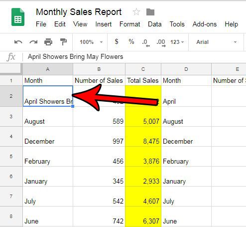
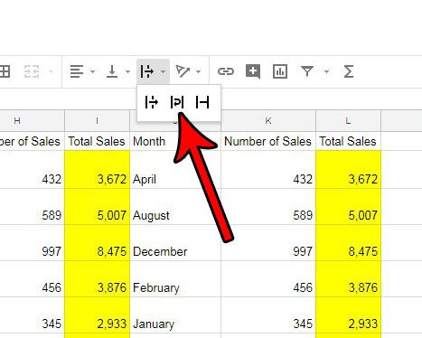
The steps in this article were performed in the desktop version of Google Chrome. This guide is going to have you select a cell containing more text than is currently visible in the cell, then changing a setting so that that overflow text is displayed on new lines in the cell. Note that this is going to increase the height of the entire row of cells in which this cell is located. Step 1: Sign into Google Drive and open the Sheets file containing the cell with the text that you wish to wrap. Step 2: Click on the cell to select it. Step 3: Select the Text wrapping button in the toolbar above the spreadsheet. Step 4: Choose the Wrap option. It’s the middle button on this dropdown menu. Do you have a row in your spreadsheet that you would prefer not be visible, but you aren’t quite ready to delete it? Find out how to hide a row in Google Sheets so that you or anyone else looking at the sheet doesn’t see the cells in that row, but you can still use those cells in formulas, or you can make that data visible in the future if you decide you need it. After receiving his Bachelor’s and Master’s degrees in Computer Science he spent several years working in IT management for small businesses. However, he now works full time writing content online and creating websites. His main writing topics include iPhones, Microsoft Office, Google Apps, Android, and Photoshop, but he has also written about many other tech topics as well. Read his full bio here.
You may opt out at any time. Read our Privacy Policy


